MSU Extension

Introduction: Crop Estimation and Vine Growth

Clear and accurate knowledge of vineyard conditions can result in long-term sustainable cultivation of grapes for juice and wine production. These conditions vary due to inconsistent weather from season to season, especially in the eastern viticultural regions of North America. Predicted climate change may increase this variability by triggering increased chances of late spring and early fall frost events; increased and variable summer heat accumulation, known as growing degree days or GDD; and increased frequency of rain events. The future economic survival and success of the grape and wine industries depends on the ability to understand the variability of these conditions and to take them into account while striving to maintain economic yields and continuing to improve fruit quality.

We’ve developed this bulletin to assist growers by providing tools to reduce both annual yield and quality variability among years, and variability due to single-year factors. Growers can achieve this reduced variability through effective, accurate crop estimation (CE). Through CE, growers can predict as accurately as possible the quantity of grapes they will harvest in any given season. This prediction is necessary (1) to achieve the agreed upon tonnage goals the purchaser sets, (2) to determine whether vines are balanced, that is, not overcropped or undercropped, so they produce both quality fruit and healthy vines each season and (3) to help processors of juice and wine anticipate the tank space needed.

Sustainable productivity of wine and juice grapes for both high-quality ripe fruit and mature wood depends on the appropriate ratio of exposed leaves to retained fruit, defined as crop load (Howell, 2001). An overcropped vine has an insufficient exposed leaf area relative to the weightretained fruit crop. This type of vine will have a detrimental effect, delaying fruit and wood maturity leading to a decrease in vine size, limiting future fruiting potential and reducing cold hardiness of both buds and wood. An undercropped vine has an excess of exposed leaf area relative to the weight of the retained fruit crop. This type of vine will have ripe fruit but will also have an excess of vegetative growth causing internal canopy shading and delayed ripening. It will be more prone to fungal diseases and have reduced fruit quality (Figure 1).

Figure 1. Effect of leaf area at veraison on sugar accumulation (indexed as ºBrix) at harvest on Concord (Vitis labrusca L.) grown for juice grape production in Michigan (Dongvillo Vineyards, Scottsdale, Mich.). Maximum sugar accumulation was obtained with ≈ 15-20 cm2 of leaf area per gram of fruit (1 cm2 = 0.15 inch2, 1 g = 0.04 oz). Increasing the ratio (>20, i.e., undercropping the vines) or decreasing the ratio (<20, i.e., overcropping the vines) has a detrimental effect on final fruit quality at harvest, reducing the sugar level (Howell and Sabbatini, 2008).

In conclusion, the challenge is to accurately predict the yield of the vines, which have been conventionally pruned, and plan crop reduction strategies if necessary. Growers must (a) predict yield per vine and (b) determine whether, when and how much fruit they should remove at thinning time. Thinning before fruit set has minimal impact on yield due to naturally occurring compensation resulting in increased fruit set and larger berries. Thinning at veraison or later reduces the crop, but allows for little increase in fruit composition or physiological maturity (Dokoozlian and Hirschfelt, 1995). The best time to adjust the crop appears to be between 20 and 30 days after bloom, typically at midpoint between fruit set and veraison for eastern viticultural production regions.

Physiology of Berry Growth

A fleshy fruit, the grape berry grows in size and weight during the season following an “S” shaped or double sigmoid curve pattern divided into three stages (Figure 2). After bloom, or flowering, and fruit set, initial berry growth includes rapid cell division and a subsequent cell expansion. The phase of cell division (STAGE I) is followed by an intermediate phase (STAGE II) of reduced growth called the lag phase and finally a phase of cell expansion (STAGE III), the ripening period when sugars and other important metabolites accumulate (Ollat et al., 2002).

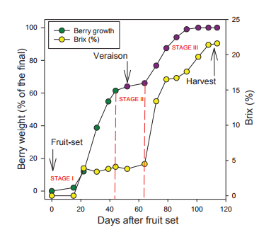
Figure 2. Berry growth (% fresh weight of final) and sugar accumulation (Brix) in Cabernet Franc from fruit set to harvest. Note the three distinctive stages (I, II and III) of the double sigmoid pattern and the rapid accumulation of sugar at the end of stage II.

Stage I: This corresponds to a phase of cell division that results in a rapid increase in berry size and weight. Soft, green seeds and hard berries, accumulating mainly organic acids, such as tartrate and malate, and minimal sugar concentration (2-4 Brix) characterize this stage. Dependent on the grape variety, this stage’s duration lasts between 4 to 10 weeks.

Stage II: At this stage, often described as a “lag phase,” a temporary reduction in berry growth, seeds start to mature, showing a change in color and increased hardness. At this stage, you can no longer cut seeds with a sharp knife. Stage II lasts 1 to 3 weeks, depending on the variety. For example, Pinot gris has a shorter stage II than that of Cabernet Franc (Figure 3). Grape skin color change signals the end of stage II and indicates the initiation of fruit ripening or veraison.

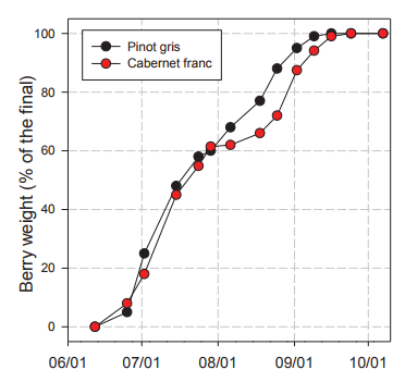
Figure 3. Berry growth in Pinot gris and Cabernet Franc during the growing season. Generally, berry growth is similar among grape varieties in stage I but differs in stage II. In this case, Pinot gris has a shorter stage II (7–10 days) than that in Cabernet Franc (15–25 days). (Adapted from Sabbatini, Tozzini, Howell, & Wolpert, 2011.)

Stage III: During this ripening period, sugars rapidly accumulate and berries soften. Here, berry volume increases rapidly, then slows until reaching a plateau a few weeks before harvest. Sugars, mainly glucose and fructose, rapidly accumulate while acids and other pigments (for example, chlorophyll) degrade. During ripening, tartaric acid is not metabolized via cellular respiration as malic acid is; therefore, its level remains relatively constant throughout this stage.

Methods of Crop Estimation

Viticulturists have developed several systems for estimating yield; we describe three in this bulletin. Growers should choose a method easy to implement for their vineyard operations.

Method 1 is based on historical records of cluster weights at harvest. Method 2 is based on cluster weights during the “lag phase,” the time during the growing season when the berry’s growth slows momentarily (around 50 to 60 days after bloom). Method 3 is based on growing degree days (GDD) accumulation and the GDD point where berry growth typically reaches approximately 50 percent of final berry weight. The formula for estimating yield of all three methods uses different systems, but all are based on (a) the number of bearing vines per acre, (b) the number of clusters per vine and (c) most noticeably, cluster weight (Hellman & Casteel, 2003; Wolpert & Vilas, 1992). Components (a) and (b) are fixed numbers during the season, while (c) is dynamic both within a season due to differences in rates of berry growth and between seasons due to differences in both spring frost incidence and conditions influencing fruit set.

Two estimation methods relate to the physiology of berry set and growth during the season and their influence on final average cluster weight. Many Oregon growers use the lag-phase crop estimation method developed for Pinot noir by Price (1992). In New York and Michigan, many juice grape growers use the GDD method developed by Pool et al. (1993) and Bates (2006). We present these methods along with our consideration of their efficacy for grapevines grown in a variable climate such as in eastern North America.

Harvest Cluster Weight Method

This simple method of estimation depends on consistent cluster weights from one season to the next. Components of yield vary each year depending on the weather, site, variety and cultural practices. You can use the following formula to estimate yield:

PY = (ANV x NC x CW) / 2000

Where:

PY = predicted yield (tons per acre)

ANV = actual number of vines per acre

NC = number of clusters per vine

CW = cluster weight (in pounds)

Components of yield influencing crop estimation:

a) Yield = tons/acre

b) Tons/acre = (yield/vine) x (# vines/acre)

c) Yield/vine = (# clusters/vine) x (cluster weight)

d) Cluster weight = (# berries/cluster) x (berry weight)

According to the formula reported above, the grower needs to measure three parameters each year: (1) the actual number of vines per acre, (2) the number of clusters per vine and (3) the cluster weight. See parameter details below:

• Actual number of vines per acre (ANV): Row and vine spacing determine the maximum number of vines per acre. For example, vineyard spacing of 6 feet by 9 feet will have 807 vines per acre. Usually, the actual number is lower than the maximum number of vines per acre due to missing vines for various reasons such as disease, winter injury, replanting or similar issues. Consequently, each year growers need to count the missing vines, and then subtract the number from the maximum number to get an accurate count of bearing vines. If 5 percent of the 807 vines per acre, or about 40 vines, were missing or nonbearing, then the ANV is 767.

• Number of clusters per vine (NC): This number will depend on how many nodes (buds) remain after winter pruning. Count clusters per vine as soon as you see them – before bloom or as late as pre-veraison. Counting clusters early when leaves don’t obscure them enhances accuracy. The number of vines on which you count clusters depends on vineyard size and uniformity. For example, you’ll need to count only 4 percent of the vines in a 1- to 3-acre vineyard with vines of uniform age and size, pruned to the same bud number. In practice, you should count a minimum of 20 vines. The higher the number of vines you select for cluster count, the more accurate your yield estimate will be. In larger, non-uniform vineyards typical of those in eastern North America, select more vines to address variability within the vineyard. In addition, select the vines methodically, for example, select every 10th vine in every other row. Select sample vines from within the vineyard to avoid an edge or borders effect. Count all the clusters on the sample vines.

• Cluster weight (CW): Cluster weight at harvest is a key part of any yield prediction program. The goal of obtaining cluster weight at harvest is not to predict the yield that year, but to provide records to facilitate yield prediction in subsequent years. The component of yield varies the most from year to year largely due to changing environmental conditions (Tables 1 and 3). For example, a spring frost kill of primary buds will reduce both cluster number per vine and the average weight of those clusters. Further, wet weather during bloom could cause poor fruit set and may lead to low cluster weight. Additionally, a dry summer tends to reduce berry weight possibly decreasing average cluster weight. Other factors that may affect cluster weight include cultural practices such as irrigation, fertilizers, vineyard floor management, incidence and severity of vine diseases, insects and wildlife. Sample clusters from vines rather than from harvest bins. You can use the same vines you used for cluster counts for cluster weights. Obtain average cluster weight by sampling at least 100 clusters throughout the vineyard, weighing the total and dividing by the number of clusters sampled. If you don’t have these data, use estimates of cluster weights shown in Table 1. Careful collection and maintenance of cluster weight records from year to year is pivotal to improve estimation. Proper record keeping will also give the grower a better sense of the annual variation related to adverse climatic conditions.

Table 1. Table 1. Average cluster weight (in pounds and grams, first and second number, respectively) of common grape varieties.*

* Sources: The Midwest Grape Production Guide, Michigan State (Dami et al., 2005) and Viticulture and Enology Program Michigan State University (unpublished data).

Example of Harvest Cluster Weight Method:

• Variety: Cabernet Franc

• Spacing = 6 x 9 feet or 807 vines/acre

• Missing/nonbearing vines = 5% or about 40 vines/acre

• Actual number of bearing vines, ANV = 807 - 40 = 767 vines/acre

• Average cluster count, NC = 40 clusters/vine

• Average cluster weight, CW = 0.23 lbs

• Predicted yield, PY = (ANV x NC x CW) / 2000 = (767 x 40 x 0.23) / 2000 = 3.5 tons/acre.

The Lag-Phase Method

Pinot noir grape growers in Oregon use the lag-phase crop estimation (CE) method. The lag-phase method presupposes the prediction of final yield on the basis that at Stage II of berry development (lag phase), berries are approximately half their final fresh weight. Seed hardness is the primary indicator that berries have entered lag phase. If the grower has an estimate of yield per vine (tons per acre) at lag phase, this allows enough time before harvest to adjust the final yield by cluster thinning, for example, to reach the desired fruit quality at harvest. The lag-phase estimate requires the measurement of the (1) number of bearing vines in the vineyard, (2) number of clusters per vine, (3) cluster weight at lag phase and (4) calculated cluster weight at harvest. This method suggests that at stage II (Figures 2 and 3), grape berries are approximately at 50 percent of their final weight. Therefore, multiplying the cluster weight by 2 gives an approximate prediction of final cluster weight at harvest. The major challenge of this method is to determine when the lag phase occurs every year. Growers need to split berries and with a sharp knife, check the resistance of the blade cutting the seeds. For Pinot noir in Oregon, the lag phase occurs approximately 55 days after bloom (Price, 1992).

Growing Degree Day (GDD) Method

Growing degree days (GDD) in eastern North America are typically calculated from April 1 to Oct. 31 with a base temperature of 50 °F (or 10 °C) as described by Baskerville and Emin (1969). Many juice grape growers use the GDD method developed for Concord in New York (Pool et al., 1993; Bates, 2006). Researchers demonstrated that berry weight of Concord at 1100 GDD, (or 1210 in Michigan, see Table 2) or approximately 30 days post bloom, reaches 50 percent of the final berry weight at harvest. Subsequent work in Michigan developed the GDD models for several other wine-grape varieties. Most varieties reach 50 percent of their berry weights when GDDs range between 1000 and 1700, which corresponds to the optimum time window for CE (Table 2).

Table 2. Growing Degree Days that correspond to 50 percent (GDD50) of harvest berry weights of common wine and juice grape varieties. Adapted from Dami and Sabbatini (2011).

*GDD – 50% computed from April 1 with 50 °F base temperature

Crop Estimaton (CE) Considerations of Methods for Eastern North American Grape Production

 1. Cluster Count Method. Employing cluster counts based only on long-term averages has an inherent weakness because it does not measure the often dramatic erratic environmental conditions and the impact of different vineyard cultural practices on cluster weight in the current season (Table 3). Even a careful collection of average cluster weight data over many years cannot account for annual fluctuations in both berry weight and number of berries per cluster common among commercial grape varieties in this region (Table 1). An annual estimate of cluster weight pre-veraison is absolutely necessary in the eastern region to achieve accurate CE. Using cluster number as a means of predicting yield can be misleading due to a wide year-to-year variance in both berry weight and number of berries per cluster.

Researchers made an annual assessment of both berry weight and berries per cluster for 6 years, from 1998 through 2003 (Table 3). The range of cluster weights was 10 to 89 grams (g) over 20 wine grape varieties. Between years 1989 through 1993, Seyval had cluster weights varying from 188 to 386 g, with the number of berries per cluster varying from 89 to 195. For Concord, years 2002 through 2005, cluster weight varied from 40 to 97 g and the number of berries per cluster was 13 to 27 (Table 3).

Table 3. Annual variation in average berry weight, average berry number per cluster and the range of cluster weights over several years of assessment. Data collected at the Southwest Michigan Research and Extension Center, Benton Harbor, Mich., from 1998 to 2003. After Howell and Clearwater (unpublished data).

1 Data collected from 1989 to 1993 at Fenn Valley Vineyards (Fennville, Mich.)
2 Data collected from 2002 to 2005 at Oxley Vineyards (Lawton, Mich.)
3 Data collected from 2000 to 2004 at Dongvillo Vineyards (St. Joseph, Mich.)

2. The Lag-Phase Method. This method of prediction is questionable for eastern viticulture as a result of the difference in the premise of timing of 50 percent final berry weight. Table 2 shows 50 percent of final cluster weight for Pinot noir was reached at 1140 GDD, or about 30 days after bloom for eastern North America. By contrast, lag phase for Pinot noir to begin at the onset of stage II, as suggested by Price (1992), is considerably later (55 days post bloom). We do not dispute that this method may work for Pinot noir in Oregon, but the data collected in eastern North America suggests it is not adaptable for use as our growing conditions are quite different and strongly influence the onset of stage II and, ultimately, final berry weight, cluster weight, vine yield and final tons per acre.

3. The Growing Degree Day Method. This method appears to hold the most promise for our growing conditions. Data taken over a range of years and varieties demonstrate the wide range of annual variability in those components influencing final average cluster weight (Table 3). Accurate estimates of berry weight and cluster weight coupled with cluster counts can allow a grower to project cropping at the highest level for a variety. When compared with the records of previous growing seasons, crop adjustments based on CE at the appropriate GDD for each grape variety will greatly improve precision of estimates for individual vineyard blocks. You can use such an approach in conjunction with initially carrying extra crop to serve as an insurance buffer against weather-induced crop reduction via either spring frost or poor fruit set. The method also allows precise adjustment of crop with follow up thinning once you know fruit set.

My Crop Estimates Are Still Off, Why?

Even with thorough sampling, accurate vine counts and many years of average cluster weight data, the actual crop tonnage at harvest can vary significantly from predicted amounts. A good CE falls within 15 percent of the actual yield. Do not get discouraged if first attempts at crop estimation are inaccurate; the more experience and data acquired, the more accurate the estimates will become. No one has more knowledge of the vineyard or a greater incentive to achieve maximum sustainable production of ripe grapes than the vineyard owner and manager. A grower is usually familiar with variability in a specific vineyard block and knows that different portions could be categorized as “high,” “moderate” or “low” producing.

We suggest that vineyard managers select a few vines characteristic of these areas. Then use them as indicators along with an estimate of vine numbers of that output category to generate an estimate of that location’s production potential for a given season. First, select a 3-vine (1-post-length) panel that accurately represents the area. Select representative, 3-vine plots for “high,” “moderate” and “low” production areas. If affordable, 6-vine plots are even more useful. Mark the vines. They serve effectively as the basis for long-term understanding of the location-vine relationship. The utility of the vineyard data grows as the information expands over the years. Developing a routine program for CE is a critical factor for future juice and wine grape production in eastern North America. It helps ensure consistent production of high-quality fruit over multiple years in our variable climate. A grape grower who is unable to invest in or elects to ignore developing operational competence in CE is likely to be at a competitive disadvantage in tightening markets.

References:

Baskerville, G. L., & Emin, P. (1969). Rapid estimation of heat accumulation from maximum and minimum temperatures. Ecology, 50, 514–517.

Bates, T. (2006). Crop load management in Western New York. Wine East. 34(4) November-December, 10–19.

Dami, I. E., Ellis, M. A., Ferree, D. C., Bordelon, B., Brown, M. V., Williams, R. N., & Doohan, D. (2005). Midwest grape production guide (Bulletin 919). Columbus, OH: The Ohio State University Extension.

Dami, I. E., & Sabbatini, P. (2011). Crop estimation of grapes (Factsheet HYG-1434-11). Columbus, OH: The Ohio State University.

Dokoozlian, N. K., & Hirschfelt, D. J. (1995). The influence of cluster thinning at various stages of fruit development on Flame Seedless table grapes. Am. J. Enol. Vitic. 46, 429–436.

Hellman, E. W., & Casteel, T. (2003). Crop estimation and thinning. In E. W. Hellman (Ed.), Oregon viticulture (1st ed.). Portland, OR: Oregon Winegrowers Association.

Howell, G. S. (2001). Sustainable grape productivity and the growth-yield relationship: A review. Am. J. Enol. Vitic. 52, 165–174.

Howell, G. S., & Sabbatini, P. (2008). Achieving vine balance with variable annual weather conditions. In Proceedings of the Midwest Grape and Wine Conference (pp. 93–103). Columbia, MO: Institute for Continental Climate Viticulture and Enology.

Ollat, N., Diakou-Verdin, P., Carde, J. P., Barrieu, F., Gaudillere, J. P., & Moing, A. (2002). Grape berry development: a review. J. Int. Sci. Vigne Vin, 36, 109–131.

Pool, R. M., Dunst, R. E., Crowe, D. C., Hubbard, H., Howard, G. E., & DeGolier, G. (1993). Predicting and controlling crop on machine or minimal pruned grapevines. In R. M. Pool (Ed.), Proceedings of the N.J. Shaulis Symposium: Pruning mechanization and crop control (pp. 31–45). Geneva, NY: New York State Agricultural Experiment Station.

Price, S. (1992). Predicting yield in Oregon vineyards. In T. Casteel (Ed.), Oregon winegrape grower’s guide (4th ed.). Portland, OR: Oregon Winegrowers Association.

Sabbatini, P., Tozzini, L., Howell, G. S., & Wolpert, J. (2011). Analysis of berry growth and maturation as related to cropping levels and seasonal variation. Proceedings of the 17th International GiESCO Symposium (pp. 239–243).

Wolpert, J. A., & Vilas, E. P. (1992). Estimating vineyard yields: Introduction to a simple, two-step method. American J. Enology and Vitic. 43(4), 384–388.

Appendix included in the PDF